Alpha testing shinyapps.io - first impressions

ShinyApps.io is a new server which is currently in alpha testing to host Shiny applications.  It is being designed by the RStudio team and provides some distinct features different from that of the ShinyApps.io is intended for larger applications and I am guessing commercial applications in the long run.  Right now it is only allowing users by invitation into their alpha program, but they are accepting applicants for beta testing.
spark.rstudio server which is intended primarily for pilot testing Shiny apps. 

The way the user interacts with the system is extremely powerful.  In the standard package for shiny it is extremely easy to experiment with applications under development by simply navigating to the directory of interest with the setwd() command then trying your app with the runApp() function in the shiny library.  The new server has its own functions including the new and extremely powerful deployApp() function which acts the same as the runApp() function except that it contacts the ShinyApps server and immediately sets up a connection and deploys your app.  This makes the entire process of developing shiny applications and deploying them much easier.

I hope that this new service will further increase the user base of shiny! I think an R based interface for generating graphs will provide an invaluable tool for teaching and demonstrating empirical analysis methods.

I have been playing around with Shiny's seeming animation functionality.  I have created an animation like interface simulating the bouncing of a ball.

http://econometricsbysimulation.shinyapps.io/bounce/

GitHub Source

A Shiny App for Experimenting with Dynamic Programming

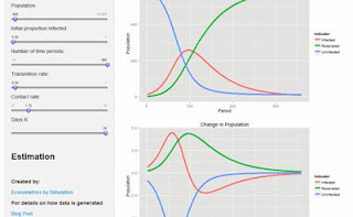
This post demonstrates the dynamics involved in a susceptible, infected, and recovering (SIR) model previous post for the model.  The shiny ui and server code can be found on GitHub.
of dynamic programming.

As a dynamic infection model, I find it particularly satisfying to be able change parameters and observe instantaneously changes in predicted outcomes.

This is a very simple model.  However, there
are many interesting models feasible that use this basic structure.  A more involved though fundamentally no more complex model might consider a simulation in which there are multiple sub-populations with different contact rates and transmission rates.  How might an optimal intervention be positioned in order to minimize total population exposure?

You can experiment with the app yourself at:

http://econometricsbysimulation.shinyapps.io/Dynamic-Pro

A Shiny App for Playing with OLS

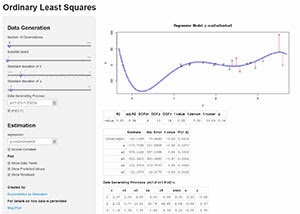
Ordinary least squares continues to be the staple estimator for causal inference for good reason.  In order to help new and veteran OLS users get a better sense of how it is working I have created a shiny app that allows for instant interactivity returning coefficient estimates and prediction graphs through Shiny's easy to use user interface controls.

The app only has a single x variable which is randomly drawn from a normal distribution with mean 2 and standard deviation specified by the user.  There is also an error term u which has mean 0 and standard deviation specified by the user.

The user also has control of how many observations to generate and how to generate the dependent variable y.

To play around with the app go to: econometricsbysimulation.shinyapps.io/OLS-App/

Source can be found on GitHub: github.com/EconometricsBySimulation/OLS-demo-App/

The Motivation for the Poisson Distribution

# The Poisson distribution has the interesting property that it
# models outcomes from events that are independent and equally
# likely to occur.  The distribution takes only one parameter mu
# which is equal to both the mean (expected number of events) 
# as well as the variance.
 
# This distribution as with all distributions is somewhat 
# fascinating because it represents an approximation of a 
# real world phenomenon.
 
# Imagine you are trying to model the mail delivery on wednesdays.
 
# On average you recieve 9 pieces of mail. If the mail delivery
# system is well modeled by a poisson distribution then
# the standard deviation of mail delivery should be 3.
# Meaning most days you should recieve between 3 and 15 pieces
# of mail.  
 
# What underlying physical phenomenon must exist for this to be
# possible?
 
# In order to aid this discussion we will think of the poisson
# distribution as a limitting distribution of the sum of 
# outcomes from a number of independent binary draws:
 
DrawsApprox <- function(mu, N) sum(rbinom(N,1,mu/N))
 
# This idea is if we specify a number of expected outcomes mu
# and give a number of draws (N>mu) then we can approximate the
# single draw of a poisson by summing across outcomes.
 
DrawsApprox(9,9)
# In this case of course the sum is 9 and variance = 0
# Under this case there are 9 letters which are always
# sent out every Wednesday.
 
# More interestingly:
DrawsApprox(9,18)
# In this case there are 18 letters that may be sent out.
# Any one of them is possible at a 50% rate.
 
# We want to know what the mean and variance is.
# Let us design a simple function to achieve this.
evar <- function(fun, draw=100, outc=NULL, ...) {
  for(i in 1:draw) outc <- c(outc, get(fun)(...))
  list(outc=outc, mean=mean(outc), var=var(outc))
}
 
evar("DrawsApprox", draw=10000, N=18, mu=9)
# I get the mean very close to 9 as we should hope
# but interestingly the variance less than five.
# This is less than that of the poisson which is 9.
 
# Let's see what happens if we double the number of
# potential letters going out which will halve the 
# probability of any particular letter.
evar("DrawsApprox", draw=10000, N=36, mu=9)
# Now the variance is about 6.7
 
evar("DrawsApprox", draw=10000, N=72, mu=9)
# Now 7.7
 
evar("DrawsApprox", draw=10000, N=144, mu=9)
# 8.6
 
evar("DrawsApprox", draw=10000, N=288, mu=9)
# 8.65
 
# We can see that as the number of letters gets very large
# the mean and variance of the number letters approaches
# the same number 9.  I will never be able to choose a 
# large enough number of letters so that the variance exactly
# equals the mean.
 
# However the didactic point of how the distribution is 
# structured and when it may be appropriate to use should be
# clear.  Poisson is a good fit when the likelihood of each
# individual outcome is equal, yet the number of possible
# outcomes is large (in principal I could recieve 100 pieces
# of mail in a single day though it would be very unlikely).
 
bigdraw <- evar("DrawsApprox", draw=10000, N=1000, mu=9)
summary(bigdraw$outc)

Created by Pretty R at inside-R.org

Batch Variable Rename - Stata

* Using macros it is very easy to rename any number of variables in Stata.

* Imagine you have a number of variables.

clear
set obs 10

forv i=1/100 {
  gen var`=`i'^2' = rnormal()
}

* We can rename variables by using a - mark which tells Stata to use
* the variable list.

foreach v of varlist var1-var100 {
  rename `v' `v'A
}

* We can also rename with the wildcards * and ?

foreach v of varlist var*4* {
  rename `v' four`v'
}

Formatted By Econometrics by Simulation

Consumer's Choosing an Optimal Bundle - Utility Maximization

# The theoretical basis of classical consumer theory lies
# in utility maximization. The idea is that consumers
# make consumption decisions based on choosing a bundle 
# of goods that will maximize individual utility.
# Despite this hypothesis being largely unsupported
# by reproducible results indicating the superiority
# any utility function over all other functions this
# theory persists.
 
# In this simulation I set up an easy framework for the 
# user to simulate the decision of the consumer as a
# function of the utility function, price of goods,
# and consumer budget.
 
 
# Uof is the function that takes a choice of
# x and y and calculates the corresponding z as
# well as expected utility.
 
Uof <- function(XY) {
  # x cannot be less than 0 or more than all of the
  # budget expended on x
  x <- min(max(XY[1],0), b/px)
  # y cannot be less than 0 or more than the remaining
  # budget left after x expenditures 
  y <- min(max(XY[2],0), (b - x*px)/py)
 
  # z is purchased with whatever portion of the budget 
  # remains
  z <- (b - x*px - y*py)/pz
 
  # Display the quantity of x,y, and z chosen.
  print(paste0("x:", x, " y:", y, " z:", z))
 
  # Since optim minimizes a function I am making
  # the returned value equal to negative utility.  
  -utility(x,y,z)
}
 
# I have defined a few different potential utility
# functions.
 
cobb.douglas2  <- function(x,y,z) x^.3*y^.3
cobb.douglas3  <- function(x,y,z) x^.3*y^.3*z^.4
lientief3      <- function(x,y,z) min(x,y,z)
linear.concave <- function(x,y,z) x^.3 + y^.2 + z^.5
mixed          <- function(x,y,z) min(x, y)^.5*z^.5
addative       <- function(x,y,z) 2*x+3*y+z
 
# Choose the utility function to maximize
utility <- cobb.douglas3
 
# Choose the prices
px <- 1
py <- 1
pz <- 1
 
# Choose the total budget
b <- 100
 
# Let's see how much utility we get out of setting
# x=1 and y=1
Uof(c(1,1))
 
# The following command will maximize the utility
# subject the choice of the utility fuction, prices,
# and budget.
optim(c(1,1), Uof, method="BFGS")
 
# In general it is a good idea not to use such 
# computational methods as this since by instead
# solving mathematically in closed form for solutions
# to utility maximization functions, you can discover
# how exactly a change in one parameter in the model
# may lead to a change in quantity demanded of a
# type of good.
 
# Of course you could do something fairly simple along
# these lines in R as well.
 
# For instance, define vectors:
 
# Once again choose what utility function
utility <- linear.concave
 
xv  <- NULL
yv  <- NULL
 
pxv <- seq(.25,10,.25)
 
for (px in pxv) {
  res <- optim(c(1,1), Uof, method="BFGS")
  xv <- c(xv, max(res$par[1],0))
  yv <- c(yv, max(res$par[2],0))
}
 
plot(xv, pxv, type="l", main="Demand for X(px)",
     xlab="Quantity of X", ylab="Price of X")
 
# The map of the demand function for X 

  
 
plot(yv, pxv, type="l", main="Demand for Y(px)",
     xlab="Quantity of Y", ylab="Price of X") 

  
# The map of the demand function for y as a function
# of the price of x. It is a little erratic probably
# because of lack of precision in the optimization
# algorithm.

Highlighted by Pretty R at inside-R.org

Efficiency Balanced Information Criterion for Item Selection

# Han (2012) in the paper "An Efficiency Balanced Information Criterion 
# for Item Selection in Computerized Adaptive Testing" proposes a method
# of evaluating potential items based on expected item potential information 
# as a function of maximum potential item information.
 
# This method favors items which have lower a values to be initially
# selected when there is greater uncertainty in the test but favors selection
# of items with higher a parameters as the test progresses.
 
# This small bit of code demonstrates how such a proceedure rescales
# item information.
 
# First we will define a few functions that we will use to construct our scale.
 
# Birbaum approximates the theta which maximizes the information function at
# a specific a, b, and c parameter level:
tmax <- function(a,b,c,D=1.7)
  b+1/(D*a)+log((1+sqrt(1+8*c))/2)
 
# For example:
tmax(a=2,b=2,c=.2)
 
# This is the item information function for a 3PL (3 parameter logistic)
iinfo <- function(theta,a,b,c,D=1.7)
  ((D*a)^2*(1-c))/((c+exp(D*a*(theta-b)))*
                 (1+exp(-D*a*(theta-b)))^2)
 
iinfo(theta=0,a=1,b=0,c=.1)
 
# Now we define a function which approximates the integration of function 
# "fun" from start to end.
integ <- function(start,end, step, fun, ...) {
  x <- seq(start+step/2,end-step/2,step)
  sum(get(fun)(x, ...)*step)
}
# As step size goes to zero the integ function approaches true integration.
# Of course that would mean infinite calculations which would be impossible
# for any computer.  Thus a larger step size is a worse approximation but
# uses less machine time.
 
# For example
a <- function(x,y) x^y
 
# Let's see
integ(0,2,.00001, "a", y=0)
integ(0,2,.00001, "a", y=1)
# Looking good.
 
# This is the big function that we are interested in:
IE <- function(thetahat,SEE,a,b,c,D=1.7,step=.001) {
  # thetahat is the current estimate of ability
  # SSE is the current standard error of the estimate
  # step is the number of steps used to estimate the integral
 
  # We calculate the item information at the current thetahat
  ii <- iinfo(thetahat,a=a,b=b,c=c,D=D)
  # Now we calculate the "max" theta value for the item.
  thetamax <- tmax(a=a,b=b,c=c,D=D)
  # Now the max information for that item.
  maxI <- iinfo(thetamax,a=a,b=b,c=c,D=D)
  # The efficient information as defined by Han at the
  # current theta is:
  ie <- ii/maxI
 
  # einfo is the expected information for a particular
  # item integrated across the range thetahat-SEE to
  # thetahat+SEE.
  einfo <- integ(thetahat-SEE*2, 
               thetahat+SEE*2, 
               step=step, 
               "iinfo",
               a=a,b=b,c=c,D=D)
 
  # Finally we can rescale the expected item information
  # by the maxI to find the expected item efficiency.
  eie <- einfo/maxI
 
  # This provides a list of returned values.
  list(eie=eie, 
       ii=ii,
       ie=ie,
       maxI=maxI, 
       thetamax=thetamax, 
       einfo=einfo)
}
 
test <- IE(0,1,a=1,b=0,c=.1,step=.001)
test
 
# Let's see this criterion in action:
theta <- seq(-3,3,.1)
 
# Make a list of returns
returns <- names(test) 
 
for(v in returns) assign(v,NULL)
 
# Let's create one last function that returns a list of 
# mappings for each of the ability levels.
 
mapping <- function(theta=seq(-3,3,.1), SEE=.5,a=1,b=0,c=.1,step=.001) {
  I1 <- list()
  for(i in 1:length(theta)) {
    res <- IE(theta=theta[i],SEE=SEE,a=a,b=b,c=c,step=step)
    for(v in returns) I1[[v]][i] <- res[[v]]
  }
  I1
}
 
# Now let's imagine five different items
I1 <- mapping(a=.5 , b=-1.5, c=.3, SEE=.5)
I2 <- mapping(a=1  , b=-1  , c=.3, SEE=.5)
I3 <- mapping(a=1.7, b=0   , c=.3, SEE=.5)
I4 <- mapping(a=1  , b=1   , c=.3, SEE=.5)
I5 <- mapping(a=1.5, b=1.5 , c=.3, SEE=.5)
 
plot(theta , I3$ii, type="n",
     main="Item Information at ThetaHat
     SEE=.5",
     xlab="ThetaHat", ylab="Information")
lines(theta, I1$ii, lwd=2, col="red")
lines(theta, I2$ii, lwd=2, col="blue")
lines(theta, I3$ii, lwd=2, col="green")
lines(theta, I4$ii, lwd=2, col="purple")
lines(theta, I5$ii, lwd=2, col="black")
# We can see that some items have much more information
# than other items such that they would almost never
# be selected.  Item 4 for instance is almost never expected
# to yeild higher information.
 


# If we are less sure of our theta estimate we may instead
# calculate our expected information.
plot(theta , I3$einfo, type="n",
     main="Expected Item Information at ThetaHat
     SEE=.5",
     xlab="ThetaHat", ylab="Information")
lines(theta, I1$einfo, lwd=2, col="red")
lines(theta, I2$einfo, lwd=2, col="blue")
lines(theta, I3$einfo, lwd=2, col="green")
lines(theta, I4$einfo, lwd=2, col="purple")
lines(theta, I5$einfo, lwd=2, col="black")
# In general this basically makes the peaks less extreme but
# does not generally favor our items with lower a values. 

# If we want to see how our expected efficiency item
# information value will do we can see that as well.
# However, before we do that imagine first each of these
# information functions divided by it's peak value.
plot(c(0,theta) , c(0,I1$eie), type="n",
     main="Expected Efficiency Item Information at ThetaHat
     SEE=.5",
     xlab="ThetaHat", ylab="Information")
lines(theta, I1$eie, lwd=2, col="red")
lines(theta, I2$eie, lwd=2, col="blue")
lines(theta, I3$eie, lwd=2, col="green")
lines(theta, I4$eie, lwd=2, col="purple")
lines(theta, I5$eie, lwd=2, col="black")
# Now we can see that item 1 (red) and 4 (purple) are favored by 
# this algorithm, though by standard item maximization or by 
# expected item maximization they would almost never have been
# chosen. 

# The authors suggest a summing or the Efficiency Information
# and that of expected information might yeild a good solution.
plot(c(0,theta) , c(0,I3$eie+I3$einfo), type="n",
     main="Expected Efficiency Item Information at ThetaHat
     SEE=.5",
     xlab="ThetaHat", ylab="Information")
lines(theta, I1$eie+I1$einfo, lwd=2, col="red")
lines(theta, I2$eie+I2$einfo, lwd=2, col="blue")
lines(theta, I3$eie+I3$einfo, lwd=2, col="green")
lines(theta, I4$eie+I4$einfo, lwd=2, col="purple")
lines(theta, I5$eie+I5$einfo, lwd=2, col="black")


# The argument is that as SEE gets small the information begins
# to look much more like that of Item Information which is
# appropropriate for later in the test.
I1 <- mapping(a=.5 , b=-1.5, c=.3, SEE=.15)
I2 <- mapping(a=1  , b=-1  , c=.3, SEE=.15)
I3 <- mapping(a=1.7, b=0   , c=.3, SEE=.15)
I4 <- mapping(a=1  , b=1   , c=.3, SEE=.15)
I5 <- mapping(a=1.5, b=1.5 , c=.3, SEE=.15)
 
plot(c(0,theta) , c(0,I3$eie), type="n",
     main="Expected Efficiency Item Information at ThetaHat
     SEE=.15",
     xlab="ThetaHat", ylab="Information")
lines(theta, I1$eie, lwd=2, col="red")
lines(theta, I2$eie, lwd=2, col="blue")
lines(theta, I3$eie, lwd=2, col="green")
lines(theta, I4$eie, lwd=2, col="purple")
lines(theta, I5$eie, lwd=2, col="black")
# Now we can see that item 1 (red) and 4 (purple) are favored by 
# this algorithm, though by standard item maximization or by 
# expected item maximization they would almost never have been
# chosen.


# The authors suggest a summing or the Efficiency Information
# and that of expected information might yeild a good solution.
plot(c(0,theta) , c(0,I3$eie+I3$einfo), type="n",
     main="Expected Efficiency Item Information at ThetaHat 
     SEE=.15",
     xlab="ThetaHat", ylab="Information")
lines(theta, I1$eie+I1$einfo, lwd=2, col="red")
lines(theta, I2$eie+I2$einfo, lwd=2, col="blue")
lines(theta, I3$eie+I3$einfo, lwd=2, col="green")
lines(theta, I4$eie+I4$einfo, lwd=2, col="purple")
lines(theta, I5$eie+I5$einfo, lwd=2, col="black")


 
# We can see that item 1 is still favored though we expected
# it to give us very little information.  Overall, the
# method seems interesting but not yet ideal.

Created by Pretty R at inside-R.org