Results of an Informal Survey of R users

# This post does some basic correlation analysis between responses
# to the survey I recently released through R Shiny at:
http://www.econometricsbysimulation.com/2013/11/Shiny-Survey-Tool.html
 
# I have saved the data from the survey after completing the survey myself.
# This data is incomplete because the survey has been running since I
# saved the survey and because shinyApp.io server automatically resets
# data every so often. Thus survey results are lost sometimes.
# (Something to be remedied at a future time.)
 
# Let's get our data
Rsurvey <- read.csv(paste0(
  "https://raw.github.com/EconometricsBySimulation/",
  "Shiny-Demos/master/Survey/sample-results.csv"))
 
summary(Rsurvey)
# Looking at the data we have 321 responses in total though
# on average it looks like we have closer to 250 responses
# to work with.
 
# The majority of respondents consider their knowledge of R
# to be either Advanced (119) or Moderate (92).
 
# The majority of users are aged 26-35 (121) or 36-45 (79).
 
# The frequency that respondents read R bloggers is
# most frequently daily (164) or weekly (75).
 
# The frequency of respondents read my blog never (149)
# or monthly (48).
 
# The self-reported technical knowledge of most users in a
# theoretic stastics/econometrics/pschometrics field was
# most frequently reported as either moderate (103) or
# advanced (97).
 
# The favorite colors of people was most frequently blue (114)
# and green (66).
 
# The vast majority of respondents were male (243) compared
# with only 22 females. Looks like R bloggers is not going
# to become a dating website in the near future.
 
# Of those who selected an area of research the majority
# chose data analysis (150) followed by (statistics).
 
# As for the user's knowledge of Shiny few had much at all with
# Basic (118) and Non (76) being the most frequent responses.
 
# Finally, as to the question of "What is the air speed velocity
# of an unladen swallow" the majority of respondents chose
# the correct response to the Monte Python reference (129)
# while the next largest group indicated that "they did not 
# know" (98).
 
# Well let's see if there is any correlation between particular
# outcomes of interest.
 
# Let's see if there is a correlation between knowledge of R
# and frequency of reading R bloggers.
knowledgeR <- rep(NA, nrow(Rsurvey))
 
knowledgeR[Rsurvey[,2]=="None"] <- 0
knowledgeR[Rsurvey[,2]=="Basic"] <- 1
knowledgeR[Rsurvey[,2]=="Moderate"] <- 2
knowledgeR[Rsurvey[,2]=="Advanced"] <- 3
knowledgeR[Rsurvey[,2]=="Expert"] <- 4
 
frequency <- rep(NA, nrow(Rsurvey))
 
# Convert these rates to number of days per year
# reading R bloggers.
frequency[Rsurvey[,5]=="None"] <- 0
frequency[Rsurvey[,5]=="daily"] <- 360
frequency[Rsurvey[,5]=="weekly"] <- 50
frequency[Rsurvey[,5]=="monthly"] <- 12
 
cor(frequency, knowledgeR, use="pairwise.complete.obs")
# There seems to be modest correlation beteen # of days spent
# reading R bloggers and self assessment of R expertise.
 
# Let's see if coldness or warmth allong the color
# spectrum is a useful variable.
warmth <- rep(NA, nrow(Rsurvey))
 
warmth[Rsurvey[,8]=="blue"] <- 0
warmth[Rsurvey[,8]=="green"] <- 1
warmth[Rsurvey[,8]=="orange"] <- 2
warmth[Rsurvey[,8]=="red"] <- 3
 
cor(warmth, knowledgeR, use="pairwise.complete.obs")
# There is a slight negative correlation between
# the favorite color warmth of users and self-reported
# knoweldge of R.
 
# Finally, let's look at success on the Monte Python
# trivia question.
monte <- rep(NA, nrow(Rsurvey))
 
monte[Rsurvey[,12]=="I don't know!"] <- 0
monte[Rsurvey[,12]=="~50 MPH"] <- 0
monte[Rsurvey[,12]==
  "What do you mean? An African or European swallow?"] <- 1
 
cor(monte, knowledgeR, use="pairwise.complete.obs")
# We see a modest positive correlation between
# knowledge of R and being able to answer Monte Python
# trivia.
 
knowledgeStats <- rep(NA, nrow(Rsurvey))
 
knowledgeStats[Rsurvey[,6]=="None"] <- 0
knowledgeStats[Rsurvey[,6]=="Basic"] <- 1
knowledgeStats[Rsurvey[,6]=="Moderate"] <- 2
knowledgeStats[Rsurvey[,6]=="Advanced"] <- 3
knowledgeStats[Rsurvey[,6]=="Expert"] <- 4
 
cor(knowledgeStats, knowledgeR, use="pairwise.complete.obs")
# There seems to be a very stong correlation with
# self reported knowledge of Statstics and knowedge
# of R.
 
# In order to see the data points a little more clearly
# I will add some tiny noise to both knowledge sets
knowledgeStatsN <- knowledgeStats + .15*rnorm(nrow(Rsurvey))
knowledgeRN <- knowledgeR + .15*rnorm(nrow(Rsurvey))
 
plot(knowledgeRN, knowledgeStatsN, 
    main="Knowledge of Stats against that of R",
    xlab="R", ylab="Stats")
# We can see the diagnol elements 2,2 and 3,3 have the most
# frequency. 

  
summary(lm(knowledgeR~warmth+frequency+monte+knowledgeStats))
# Overall, we can see that knowledge of Statistics
# stongly positively predicts knowledge of R.
# Frequency of reading R bloggers also seems to
# have an effect size significant nearly at the
# %5 level.
 
# The coefficient on frequency is very small but that is because
# the scale is quite large (from 0 to 360).  However
# if someone where to start reading R bloggers daily
# (assuming R-bloggers -> R knowledge one directionally)
# Then we would expect a change of R knowledge of:
.0006994*360
# 0.251784
 
# Not as large a predictor as knowledge of stats but certainy
# there exists some relationship.
 
# Of course little causal relationships can be inferred from the
# data.  We cannot expect reading R bloggers to be independent
# of self-assessed knowledge of R any more than knowledge of 
# statistics to be uncorrelated with knowledge of R since
# many users, learn R simultaneously with statistics.

Created by Pretty R at inside-R.org

Raising Statistical Standards Effect on Sample Size

The failure of mainstream research to consistently reproduce results have led many to look for the faults in current methodologies.

One of these potential faults identified is that the significance levels of current standards is too high.  A standard rejection rate of either .05 or .01 is not high enough.

Statistician Valen Johnson recently released an article in The National Proceedings Academy of Sciences which reccomends more appropriate standard of rejection being .005 or .001.

In this post I will attempt to examine how such a change could affect the required sample size for studies.

Before initiating an experimental study often a power analysis is done.  When possible it is using a relatively simple closed form numerical statistic. This is the case when relatively simple methods are intended to be used.  More complex methods often require the use of simulations to do a power analysis.

Usually the logic of a power analysis (as far as I know) goes something like.  Let's say the possible effect size is tau and we know the conditional distribution of outcomes (from previous work) has a standard deviation of SD. How many people would be need to reject the null at our intended level.

Referencing wikipedia:

With Pi being power and tau being effect size and alpha being rejection power.  Assuming lots of normality:

Pi(tau) = 1 - PDFNORMAL(Z(alpha)-tau*N^.5/SD)

We want to solve for N:

# PDFNORMAL^(-1)(1 - Pi) =  Z(alpha)-tau*N^.5/SD

# tau*N^.5/SD = PDFNORMAL^(-1)(1 - Pi) - Z(alpha)

# N = ((SD/tau)*(PDFNORMAL^(-1)(1 - Pi) - Z(alpha)))^2

samp.power <- alpha="" function="" p="" pi="" tau="">

  ceiling(((SD/tau)*(pnorm(1 - pi) - qnorm(alpha)))^2)

# added the ceiling function to round up.

Let's see it in action!

Let's say we have an outcome which we know has a SD=2 and we hope our effect will have at least a size of tau=1. Following standard practices we require a detection rate of 80% for our power analysis.  Let's see what happens when we vary our alpha rate!

samp.power(SD=2, tau=1, pi=.8, alpha=.05)

# 20

samp.power(SD=2, tau=1, pi=.8, alpha=.01)

# 34

samp.power(SD=2, tau=1, pi=.8, alpha=.005)

# 40

samp.power(SD=2, tau=1, pi=.8, alpha=.001)

# 54

We can see that increasing our rejection standards from .05 to .001 we are basically increasing our required sample pool by 2.7. Which is really not that bad.  Looking at a smaller effect size does not change things except by a squared factor s. tau'=tau/s

# Looking at our equation for N

# N = ((SD/tau)*(pnorm(1 - pi) - qnorm(alpha)))^2

# N = (1/tau * H)^2

# where H = (SD)*(pnorm(1 - pi) - qnorm(alpha))

# Thus substituting in tau'

# N = (1/tau/s * H)^2 = s^2 * (H/tau)^2

# So let's say s=10 then N(tau')=N(tau)*100

samp.power(SD=2, tau=1/10, pi=.8, alpha=.001)

# 5387

Not to make light of this new proposed rejection rate and its larger sample size.  By increasing the sample size by roughly a factor of 2.7 the cost of a study might easily double.

However, a researcher saying that the chance of an outcome occurring randomly going from 1 out of 20 to 1 out of 1000 might easily be worth the additional cost.

The nice thing about this new approach would be that it would still allow for less strong rejections even when the effect size is smaller than expected or when there is more noise in the sample than expected.

Well, that is what I have to say in support of the idea.  I also have some reservations.  If the cost of the larger rejection rates is really doubling the cost of the study then why not do two studies?  Assuming the outcomes of each study are random and iid the likelihood of rejecting the null 1 out of 20 (5%) of the time given two studies is 1 out of 20^2 or 1 out of 400.

.25% (1/400) is not as good as as .1% but it is still pretty strong.

It makes sense in a world where we do not know what really has an effect to have more smaller studies which we follow up with larger studies when we do find an effect.  In addition, there might be factors unique to individual studies which are for whatever reason unobservable and nonreproducable, driving the results.

Say, the researchers introduced bias without intending to.  Scaling up the project might have no effect on removing or controlling that bias.  However, having two different studies run by different research groups is less likely to reintroduce the same bias.

Overall, I think it may be useful to introduce higher standards into social science research especially in non-experimental data in which numerous potential researchers are looking at the data with different hypothesizes.  It is improbable that if there is enough researchers looking at the data from enough angles that there will not be at least a few that reject at a 5% level.  Imagine that you have 20 research teams each picking 5 different angles that is 1000 different draws. 

Assuming they are independent the likelihood of rejecting at a 5% level would lead researchers to falsely reject 50 null hypothesizes on average.  That is a lot of false rejections.  Choosing a level of .1% however would lead only one research team to reject one null falsely on average.  This is a pretty appealing change for a conservative statistician.   However, once again there will be many times in which we fail to reject the null when our hypothesizes are in fact true but our data or effect set are insufficiently large.  Which would we rather we have?

A Survey Tool Designed Entirely in Shiny Surveying Users of R

I have written a very basic survey tool built entirely in the Shiny package of R.  I hope the tool is useful.  Modifying the survey for your own purposes is trivially easy (I hope).


I have not commented my code so it is pretty messy right now.  You can find the source on GitHub.

In order to run your own survey all you need do is edit the Qlist.csv file.  It contains one row for each question and one column for the question text and additional columns for potential answers (which will enter the radio buttons).  All of the questions will have the default option of "Prefer not to answer" selected.  It should be easy to modify this option as well since you need only find where this text appears in the server.R code.

It should be equally easy to change the introductory message and the accreditation to me, though it would be nice if you left a link somewhere back to me.

I will comment the GitHub files as soon as I have chance.  If people find this tool useful perhaps I will work on improving it.  Please tell me if you find it useful or have suggestions for future improvements!

Please take note that it is really not up in running in a sustainable way since I was recently told that sometimes the ShinyApps.io server must be restarted which means that all of the files are restored to those when the app was originally set up.


http://econometricsbysimulation.shinyapps.io/Survey/

Alpha testing shinyapps.io - first impressions

ShinyApps.io is a new server which is currently in alpha testing to host Shiny applications.  It is being designed by the RStudio team and provides some distinct features different from that of the ShinyApps.io is intended for larger applications and I am guessing commercial applications in the long run.  Right now it is only allowing users by invitation into their alpha program, but they are accepting applicants for beta testing.
spark.rstudio server which is intended primarily for pilot testing Shiny apps. 

The way the user interacts with the system is extremely powerful.  In the standard package for shiny it is extremely easy to experiment with applications under development by simply navigating to the directory of interest with the setwd() command then trying your app with the runApp() function in the shiny library.  The new server has its own functions including the new and extremely powerful deployApp() function which acts the same as the runApp() function except that it contacts the ShinyApps server and immediately sets up a connection and deploys your app.  This makes the entire process of developing shiny applications and deploying them much easier.

I hope that this new service will further increase the user base of shiny! I think an R based interface for generating graphs will provide an invaluable tool for teaching and demonstrating empirical analysis methods.

I have been playing around with Shiny's seeming animation functionality.  I have created an animation like interface simulating the bouncing of a ball.

http://econometricsbysimulation.shinyapps.io/bounce/

GitHub Source

A Shiny App for Experimenting with Dynamic Programming

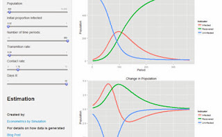
This post demonstrates the dynamics involved in a susceptible, infected, and recovering (SIR) model previous post for the model.  The shiny ui and server code can be found on GitHub.
of dynamic programming.

As a dynamic infection model, I find it particularly satisfying to be able change parameters and observe instantaneously changes in predicted outcomes.

This is a very simple model.  However, there
are many interesting models feasible that use this basic structure.  A more involved though fundamentally no more complex model might consider a simulation in which there are multiple sub-populations with different contact rates and transmission rates.  How might an optimal intervention be positioned in order to minimize total population exposure?

You can experiment with the app yourself at:

http://econometricsbysimulation.shinyapps.io/Dynamic-Pro

A Shiny App for Playing with OLS

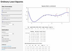
Ordinary least squares continues to be the staple estimator for causal inference for good reason.  In order to help new and veteran OLS users get a better sense of how it is working I have created a shiny app that allows for instant interactivity returning coefficient estimates and prediction graphs through Shiny's easy to use user interface controls.

The app only has a single x variable which is randomly drawn from a normal distribution with mean 2 and standard deviation specified by the user.  There is also an error term u which has mean 0 and standard deviation specified by the user.

The user also has control of how many observations to generate and how to generate the dependent variable y.

To play around with the app go to: econometricsbysimulation.shinyapps.io/OLS-App/

Source can be found on GitHub: github.com/EconometricsBySimulation/OLS-demo-App/

The Motivation for the Poisson Distribution

# The Poisson distribution has the interesting property that it
# models outcomes from events that are independent and equally
# likely to occur.  The distribution takes only one parameter mu
# which is equal to both the mean (expected number of events) 
# as well as the variance.
 
# This distribution as with all distributions is somewhat 
# fascinating because it represents an approximation of a 
# real world phenomenon.
 
# Imagine you are trying to model the mail delivery on wednesdays.
 
# On average you recieve 9 pieces of mail. If the mail delivery
# system is well modeled by a poisson distribution then
# the standard deviation of mail delivery should be 3.
# Meaning most days you should recieve between 3 and 15 pieces
# of mail.  
 
# What underlying physical phenomenon must exist for this to be
# possible?
 
# In order to aid this discussion we will think of the poisson
# distribution as a limitting distribution of the sum of 
# outcomes from a number of independent binary draws:
 
DrawsApprox <- function(mu, N) sum(rbinom(N,1,mu/N))
 
# This idea is if we specify a number of expected outcomes mu
# and give a number of draws (N>mu) then we can approximate the
# single draw of a poisson by summing across outcomes.
 
DrawsApprox(9,9)
# In this case of course the sum is 9 and variance = 0
# Under this case there are 9 letters which are always
# sent out every Wednesday.
 
# More interestingly:
DrawsApprox(9,18)
# In this case there are 18 letters that may be sent out.
# Any one of them is possible at a 50% rate.
 
# We want to know what the mean and variance is.
# Let us design a simple function to achieve this.
evar <- function(fun, draw=100, outc=NULL, ...) {
  for(i in 1:draw) outc <- c(outc, get(fun)(...))
  list(outc=outc, mean=mean(outc), var=var(outc))
}
 
evar("DrawsApprox", draw=10000, N=18, mu=9)
# I get the mean very close to 9 as we should hope
# but interestingly the variance less than five.
# This is less than that of the poisson which is 9.
 
# Let's see what happens if we double the number of
# potential letters going out which will halve the 
# probability of any particular letter.
evar("DrawsApprox", draw=10000, N=36, mu=9)
# Now the variance is about 6.7
 
evar("DrawsApprox", draw=10000, N=72, mu=9)
# Now 7.7
 
evar("DrawsApprox", draw=10000, N=144, mu=9)
# 8.6
 
evar("DrawsApprox", draw=10000, N=288, mu=9)
# 8.65
 
# We can see that as the number of letters gets very large
# the mean and variance of the number letters approaches
# the same number 9.  I will never be able to choose a 
# large enough number of letters so that the variance exactly
# equals the mean.
 
# However the didactic point of how the distribution is 
# structured and when it may be appropriate to use should be
# clear.  Poisson is a good fit when the likelihood of each
# individual outcome is equal, yet the number of possible
# outcomes is large (in principal I could recieve 100 pieces
# of mail in a single day though it would be very unlikely).
 
bigdraw <- evar("DrawsApprox", draw=10000, N=1000, mu=9)
summary(bigdraw$outc)

Created by Pretty R at inside-R.org